
Geophysical Methods
Gravity Methods
Gravity methods measure the acceleration of a gravitation field. A gravimeter (or gravity meter) is a passive, low-impact, non-invasive geophysical tool (OpenEI) that measures and maps lateral changes in the Earth's gravity field, which is a function of Earth material (e.g., rock type) density differences. Gravimeters can be deployed on the ground surface, from the air, in water, or via a borehole tool to collect data on density distribution in the subsurface (OpenEI). Because rock types have different densities, gravity data can be used to identify changes in stratigraphy. Stratigraphic information derived from gravity surveys can be used to develop the conceptual site model (CSM) for a contaminated site1. Technological advances in satellite altimetry, synthetic aperture radar interferometry, and digital terrain models have facilitated the use of rapid airborne and satellite-based gravity surveys.
| Density | |||
| Rock Type | Number of Samples | Mean (kg/m3) | Range (kg/m3) |
| Igneous Rocks | |||
| Granite | 155 | 2,667 | 2,516-2,809 |
| Granodiorite | 11 | 2,716 | 2,668-2,785 |
| Syenite | 24 | 2,757 | 2,630-2,899 |
| Quartz Diorite | 21 | 2,806 | 2,680-2,960 |
| Diorite | 13 | 2,839 | 2,721-2,960 |
| Gabbro (olivine) | 27 | 2,976 | 2,850-3,120 |
| Diabase | 40 | 2,965 | 2,804-3,110 |
| Peridotite | 3 | 3,234 | 3,152-3,276 |
| Dunite | 15 | 3,277 | 3,204-3,314 |
| Pyroxenite | 8 | 3,231 | 3,100-3,318 |
| Anorthosite | 12 | 2,734 | 2,640-2,920 |
| Rhyolite obsidian | 15 | 2,370 | 2,330-2,413 |
| Basalt glass | 11 | 2,772 | 2,704-2,851 |
| Sedimentary Rocks | |||
| Sandstone | |||
| St. Peter | 12 | 2,500 | |
| Bradford | 297 | 2,400 | |
| Berea | 18 | 2,390 | |
| Cretaceous, Wyo | 38 | 2,320 | |
| Limestone | |||
| Glen Rose | 10 | 2,370 | |
| Black River | 11 | 2,720 | |
| Ellenberger | 57 | 2,750 | |
| Dolomite | |||
| Beckmantown | 56 | 2,800 | |
| Niagara | 14 | 2,770 | |
| Marl | |||
| Green River | 11 | 2,260 | |
| Shale | |||
| Pennsylvanian | 2,420 | ||
| Cretaceous | 9 | 2,170 | |
| Metamorphic Rocks | |||
| Gneiss (Vermont) | 7 | 2,690 | 2,660-2,730 |
| Schists | |||
| Quartz-mica | 76 | 2,820 | 2,700-2,960 |
| Muscovite-biotite | 32 | 2,760 | |
| Chlorite-sericite | 50 | 2,820 | 2,730-3,030 |
| Slate (Taconic) | 17 | 2,810 | 2,710-2,840 |
| Amphibolite | 13 | 2,990 | 2,790-3,140 |
| Unconsolidated Sediment | |||
| Silt (loess) | 3 | 1,610 | |
| Sand | |||
| Fine | 54 | 1,930 | |
| Very fine | 15 | 1,920 | |
| Silt-sand-clay | |||
| Hudson River | 3 | 1,440 | |
Surface-based surveys collect gravity data using a gravimeter, which is a highly sensitive spring balance.2 In gravity surveys, the local acceleration of gravity is measured in units of Gal (after Galileo). One Gal is equal to an acceleration of 1 cm/s2. Most measurements of the difference between the Earth's normal gravity field and that observed at the ground surface are on the order of several milliGals (mGals) (Zohdy et al., 1974![]() ). Microgravimeters that measure in units of microGals (µGals) are sensitive enough to identify near-surface features such as buried channels, bedrock structural features, voids, caves, low-density zones in foundations, and underground storage tanks (ASTM 2018).
). Microgravimeters that measure in units of microGals (µGals) are sensitive enough to identify near-surface features such as buried channels, bedrock structural features, voids, caves, low-density zones in foundations, and underground storage tanks (ASTM 2018).
Typical Uses
Gravity survey measurements can be used to (OpenEI):
- Determine lithology (rock type may be inferred from differences in density).
- Identify geologic discontinuities such as joints or faults.
- Detect void spaces, and buried channels in rock formations.
- Ascertain aquifer dimensions and heterogeneities.
- Monitor groundwater table changes over time.
- Calculate large-scale water balance for applications in reservoir and aquifer management.
- Monitor changes in glacial mass related to climate change.
Understanding lithology and stratigraphy at a contaminated site is critical to identifying potential contaminant migration pathways. For example, gravimetry can identify buried faults and void spaces in rock or deposits of former river or stream channels that can serve as preferential pathways for dissolved contaminants (AAPG Wiki).
Figure 1. Time lapse of microgravity monitoring of artificial recharge as part of the Southern Avra Valley Storage and Recovery Project (U.S. Geological Survey, 2013).
For water resource studies, such as artificial recharge to aquifers, the ability to measure aquifer thickness is important. Figure 1 is a time-lapse compilation of an artificial recharge study conducted by the U.S. Geological Survey of the Southern Avra Valley Storage and Recovery Project (SAVSARP) (USGS 2013).
↩Theory of Operation
The gravimetric geophysical method is based on two laws of physics: the Law of Universal Gravitation3 and Newton's Second Law of Motion4 (Zohdy, et al., 1974![]() ). Any object with mass on the Earth's surface will be attracted to the Earth by a force, the object's weight. If the object is elevated a short distance above the Earth and allowed to drop, it will fall with gravitational acceleration. The acceleration is a function of both the mass of the Earth and the distance to the Earth's center (the shell theorem). This principle also applies to geologic bodies in the subsurface. Gravimeters on the ground surface measure the sum of the attractions of the underlying geologic body and the rest of the Earth. If the underlying geologic body is more dense than surrounding geology, it will produce a higher gravimeter reading; if it is less dense, it will produce a lower reading.
). Any object with mass on the Earth's surface will be attracted to the Earth by a force, the object's weight. If the object is elevated a short distance above the Earth and allowed to drop, it will fall with gravitational acceleration. The acceleration is a function of both the mass of the Earth and the distance to the Earth's center (the shell theorem). This principle also applies to geologic bodies in the subsurface. Gravimeters on the ground surface measure the sum of the attractions of the underlying geologic body and the rest of the Earth. If the underlying geologic body is more dense than surrounding geology, it will produce a higher gravimeter reading; if it is less dense, it will produce a lower reading.
System Components
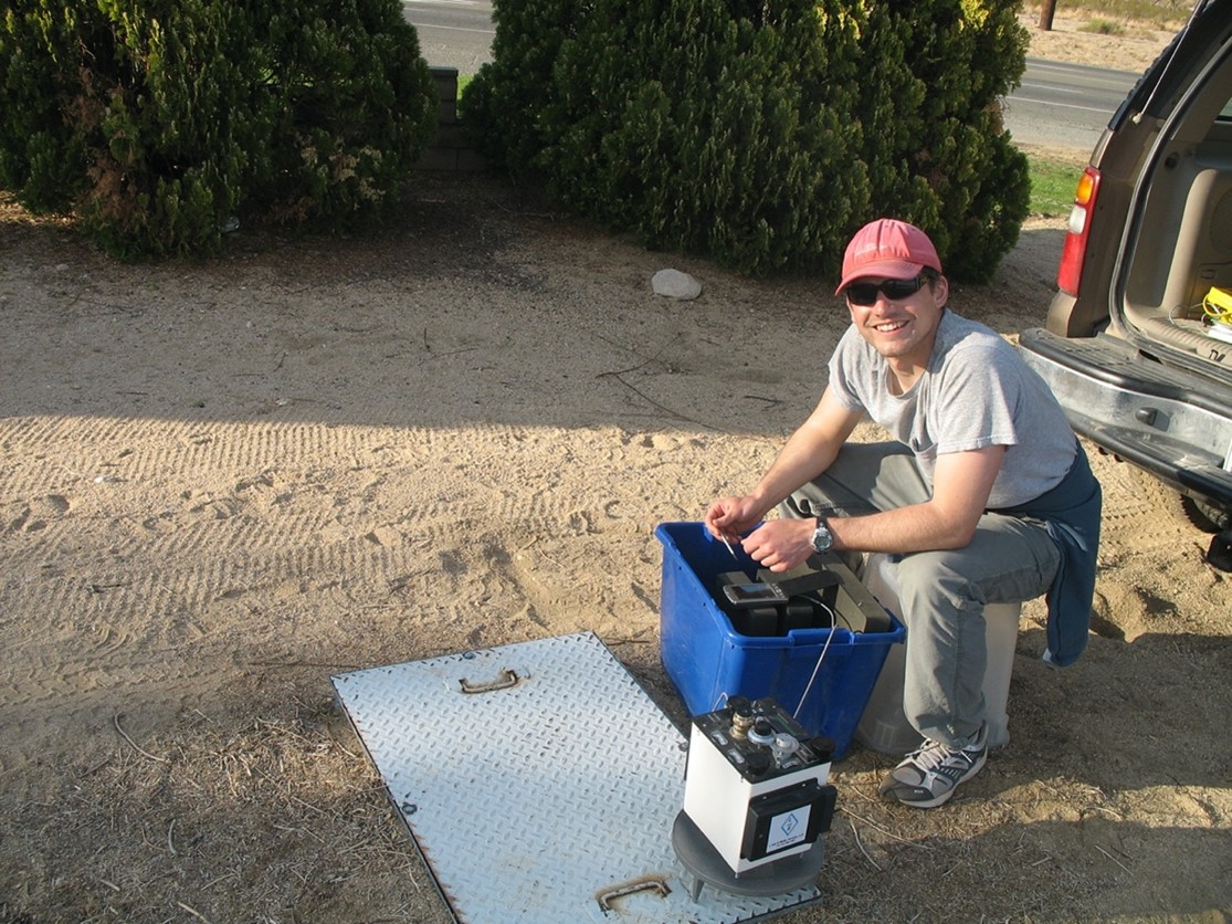
Figure 2. A USGS hydrologist prepares equipment to conduct a gravity survey to evaluate small variations in the Earth's gravity field (U.S. Geological Survey,2007).
A gravimeter uses two categories of measurement: relative and absolute. The most commonly used instrument, the spring balance gravimeter (made with either metal or quartz springs [Nabighian, et al., 2005]), is a relative measurement device. It measures: 1) spatial differences in the gravity field between pairs of stations; or 2) temporal differences at a single point. The typical spring balance gravimeter consists of a small internal mass suspended from a spring. The mass is constant, but the weight changes at different points along the Earth, varying with the local acceleration due to gravity (Zohdy et al., 1974![]() ). Figure 2 shows a small, portable field gravimeter.
). Figure 2 shows a small, portable field gravimeter.
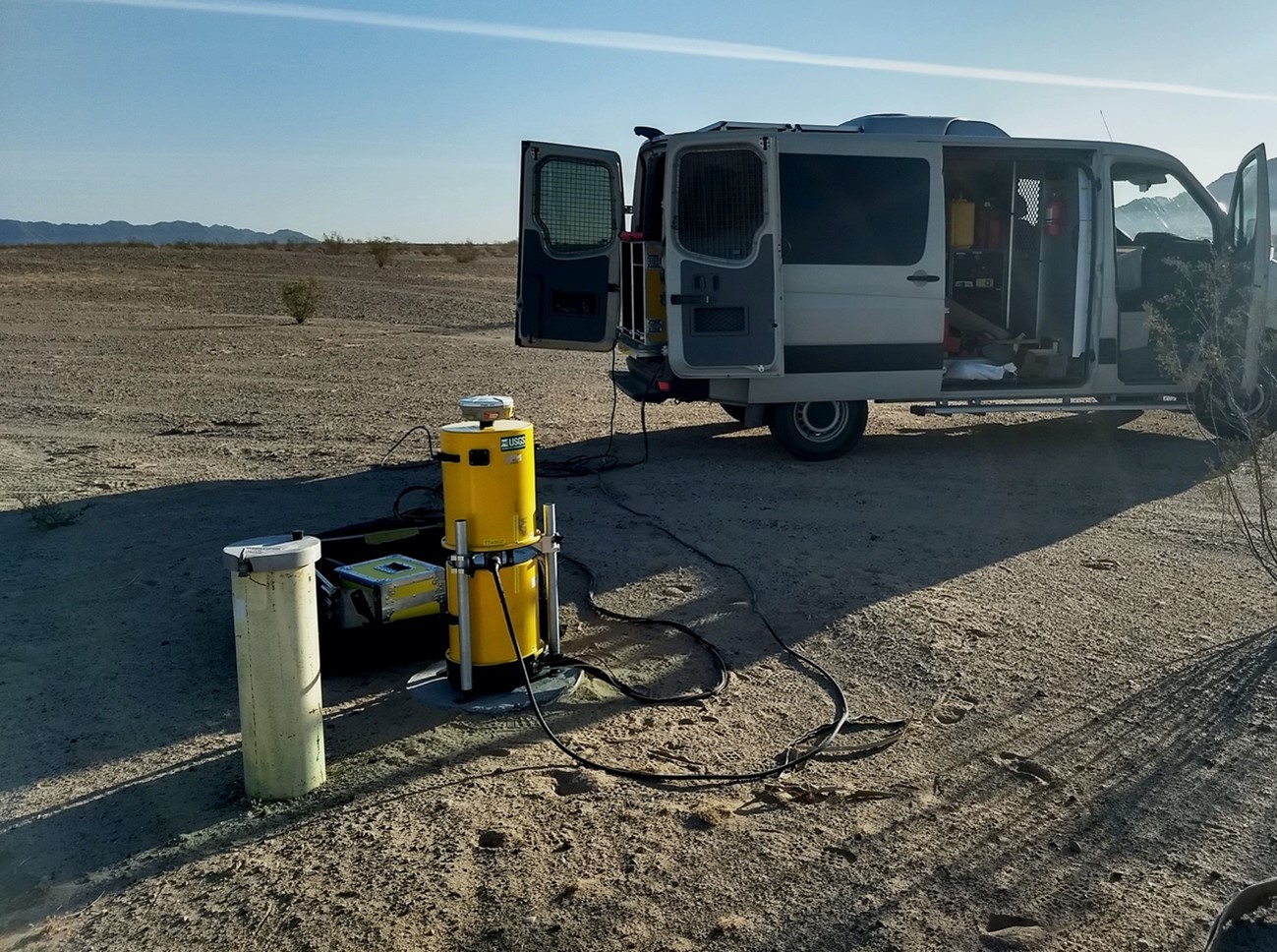
Figure 3. An example of an absolute gravity meter deployed to collect data during an aquifer storage study (U.S. Geological Survey, 2018).
Conversely, an absolute gravimeter measures the acceleration of a mass falling in a vacuum. It then calculates the absolute force of gravity at a single station over time (Carbone et al., 2020![]() ), which is useful for evaluating changes in water storage over time, or direction of water flow. This meter is not moved from station to station as with the spring gravity meter. Figure 3 shows an example of an absolute gravity meter deployed to monitor changes in groundwater storage; a laser interferometer5 measures distance, and an atomic oscillator measures time.
), which is useful for evaluating changes in water storage over time, or direction of water flow. This meter is not moved from station to station as with the spring gravity meter. Figure 3 shows an example of an absolute gravity meter deployed to monitor changes in groundwater storage; a laser interferometer5 measures distance, and an atomic oscillator measures time.
Other system components, depending on the type of gravity meter used, may include cables to connect the unit to a laptop or tablet for interfacing with the unit, and a GPS to accurately locate the position and elevation of the station (Murray and Tracey, 2001![]() ).
).
Modes of Operation
Gravity data can be collected on the ground surface, via airborne platforms (helicopter, airplane, satellite), or on waterborne platforms. Contaminated groundwater sites primarily rely on ground surface-based instruments using spring gravimeters or absolute meters as described above. A moving platform (for example a truck, helicopter, plane, ship, or satellite) gravity instrument is used to survey large or remote areas. When gravity data are collected using a moving platform, corrections must be made for the Coriolis acceleration based on the direction of the moving vehicle relative to the Earth's rotation, in addition to standard corrections.
Survey coverage will be site-specific, but depends on the station spacing, survey area conditions, and base station locations. Mapping of regional geologic structures uses widely spaced stations 30 to 300 meters apart, whereas microgravity measurements use more closely spaced measurements (e.g., 2 to 15 meters apart) to characterize localized geologic conditions (ASTM, 2020). Typically, data can be collected from 20-25 stations per day on a large-scale survey, and more for smaller-scale areas. A borehole gravimeter is sometimes used in oilfield applications to collect data on formation density as a function of depth. It is an uncommon tool for contaminated site investigations as the borehole must have a minimum diameter of at least 5½ inches (Nabighian et al., 2005).
↩Data Display and Interpretation
As described in Murray and Tracey (2001), general rules for interpreting gravity data include:
- Objects with higher-than-average mass will cause a positive gravity anomaly, the amplitude of which will be proportionate to the mass excess.
- Objects that have a lower mass than average will cause a negative anomaly.
- The dimensions of the body causing the signature will be reflected in the areal extent of the anomaly.
- Shallow targets are usually indicated by a sharp, high spring oscillation frequency anomaly.
- Deep bodies are usually represented by a broad, low-frequency anomaly.
- An estimate of the depth to the target/body can be calculated by taking half the width of the straight slope (between the points of maximum curvature) of the anomaly in its profile.
Before gravity data are integrated and presented, the data undergo several steps:
Reduction/correction – There are several types of corrections that must be applied to the raw gravity data in order to determine real anomalies indicative of changes in lithology and other hydrogeologic features. Reduction of gravity data refers to the application of corrections that remove unwanted effects that distort the gravity field of the object surveyed. Most of these corrections are made automatically with GPS data or with user input into the inversion program.
| Correction | Definition | Key Input Parameter(s) |
| Latitude | Gravity varies with latitude. Gravity is higher at the poles than at the equator. Latitude correction is determined from either a table of values at discrete increments of latitude or by using computer software packages. The latitude of each station must be known within 500 feet of its actual location to obtain an accuracy of 0.1 mGal. To obtain an accuracy of 0.01 mGal, the station location must be known to within 50 feet (Zohdy et al., 1974 |
Latitude |
| Coriolis | When gravity data are collected using a moving platform, such as an airplane, the acceleration of the vehicle will distort the measurement. A correction can be applied if the vehicle is moving at a constant speed (Murray and Tracey, 2001 |
Speed of the vehicle |
| Free air | The free air effect is a function of the elevation of the gravity station above the datum (usually mean sea level). It is caused by the variations in measured acceleration of gravity as the gravity meter is moved up and down in elevation over the irregular terrain of the Earth's surface. Changes in the distance to the center of Earth's mass will cause changes in the measured acceleration of gravity. The average value of free air change in gravity is 0.0941 mGal/foot. The free air correction is usually combined with the Bouguer Correction in most computations (Zohdy et al., 1974 |
Elevation |
| Tidal | Both the sun and the moon exert an attraction on the gravity meter in a similar fashion as they do on large bodies of water. This attraction varies with latitude and time. The maximum amplitude of the tidal effect is 0.2 mGal. The maximum rate of change is approximately 0.05 mGal/hour. Tidal effects only need to be considered and corrected for if the margin of error needs to be less than 0.2 mGal (Zohdy et al., 1974 |
Tidal variations and instrument drift. |
| Bouguer | The Bouguer effect is a function of the elevation of the gravity station above the datum (usually mean sea level). This correction is necessary because of the presence of rock between the gravity station and the datum (commonly mean sea level). The correction assumes an infinite slab of rock with a thickness equal to the height of the station above the datum exists between the station and the datum. If mean sea level is used as the datum, the elevation of the station is the thickness of the slab. The gravitational acceleration due to the infinite horizontal slab is calculated and then subtracted from the measured gravity data (Zohdy et al., 1974 |
Elevation & surface density |
| Terrain | Terrain that projects above the elevation of the gravity station exert an upward gravitational attraction. This reduces the gravity value read at the station. In addition, topographic lows such as valleys next to the station are artificially "filled" with rock in the Bouguer correction, which also reduces the resultant gravity measurement. The terrain correction is always positive regardless of whether it is for hills or valleys (Zohdy et al., 1974 |
Detailed topography & surface density |
| Drift | Most gravity meters are made of materials that are susceptible to elastic and inelastic stresses due to exposure to thermal or mechanical stresses. These stresses can cause differences in the gravity reading at the same station using the same meter but at different times. These differences are called instrument drift. Instrument drift can be accounted for by returning to the base station location routinely throughout the survey to recalibrate the instrument. Corrections to the field stations are made using the drift data collected at the base station (Zohdy et al., 1974 |
|
| Drift Eötvös | The Eötvös correction is applied only if gravity data are collected from a mobile vehicle, such as a plane or helicopter, that is moving in an east-west traverse (SEG Wiki). | Platform's velocity & heading |
Filtering and enhancement – Filtering and enhancement techniques are often built into inversion software and are used to isolate or enhance gravity anomalies of interest in the observed data. These techniques are discussed in detail in Nabighian, et al. (2005) and include:
- Regional-residual separation.
- Upward-downward continuation.
- Derivative-based filters.
- Analytical signal.
- Matched filtering.
- Wavelets.
Data interpretation – Interpretation techniques of gravity data are discussed in detail in Nabighian, et al. (2005) and include:
- Terracing.
- Density mapping.
- Forward modeling.
- Gravity inversion.
Geologic interpretation – Using data filtering techniques, portions of the gravity anomaly of interest are isolated. These target signatures are then used with other geologic information, such as established correlations between rock properties and gravity signatures, to create a model of the subsurface (Nabighian, et al., 2005).
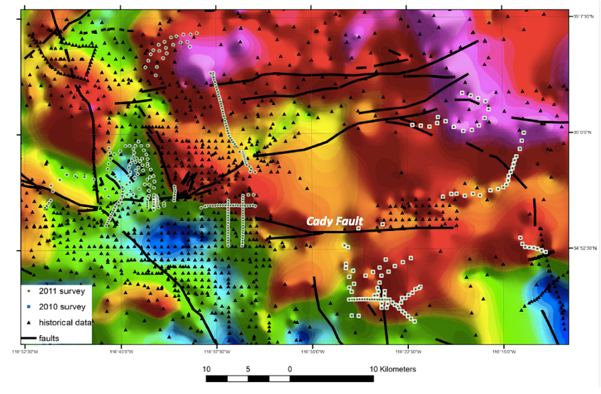
Figure 4. Isostatic residual gravity surface interpolated from historical and more recently collected data for Barstow, California. Cool colors indicate lower isostatic residual gravity (such as lower-density, unconsolidated, or partly consolidated alluvial sediments) while warm colors indicate higher isostatic residual gravity (such as denser bedrock) (Phelps, G. et al., 2013![]() ).
).
The display of the interpreted data may use 2- and 3-dimensional modeling software to incorporate other geologic information (e.g., seismic, magnetic, structural) into the visualization of the data. Geographic information systems (GIS) are used to aid in the integration of the data (Nabighian, et al., 2005).
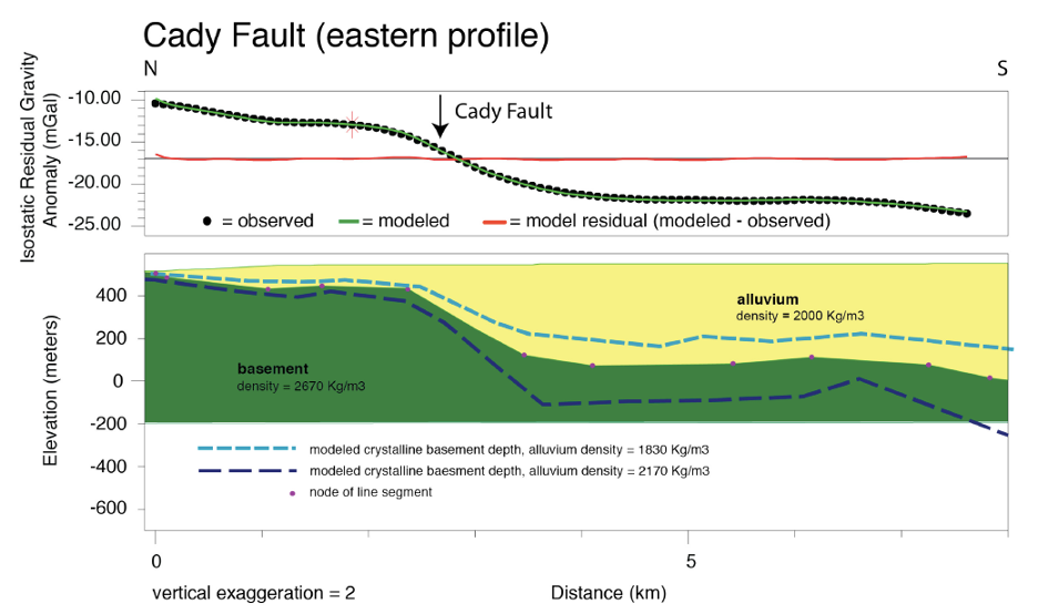
Figure 5. The modeled cross-section across the Cady Fault in Barstow, California, reveals topographic displacement in the bedrock, which likely represents fault offset. Dashed lines show how uncertainty in density values may affect the modeled alluvial sediments (Phelps, G. et al., 2013![]() ).
).
Gravity data can be used to refine the understanding of site geology and hydrogeology. For example, as described in Phelps, G., et al., (2013![]() ), mapping of the Quaternary geology in the eastern Mohave Desert identified a series of Quaternary faults with strike directions suggesting structural complexity not indicated by existing tectonic models. Further mapping of the faults was complicated by lack of surface exposures, so gravimetry was used to trace the faults beneath the Quaternary sediments. Figure 4 shows the isostatic6 residual gravity surface interpolated from historical data and data collected in 2010 and 2011 in Barstow, California. Quaternary faults are shown in black. Figure 5 shows the modeled cross-section across the Cady Fault in Barstow. Using the two in concert helps to refine the understanding of the complex geology and structure of the subsurface (Phelps, G. et al., 2013
), mapping of the Quaternary geology in the eastern Mohave Desert identified a series of Quaternary faults with strike directions suggesting structural complexity not indicated by existing tectonic models. Further mapping of the faults was complicated by lack of surface exposures, so gravimetry was used to trace the faults beneath the Quaternary sediments. Figure 4 shows the isostatic6 residual gravity surface interpolated from historical data and data collected in 2010 and 2011 in Barstow, California. Quaternary faults are shown in black. Figure 5 shows the modeled cross-section across the Cady Fault in Barstow. Using the two in concert helps to refine the understanding of the complex geology and structure of the subsurface (Phelps, G. et al., 2013![]() ).
).
Performance Specifications
Precision and accuracy of gravity methods for subsurface characterization have improved over time and are based on the parameters described below. Resolution of gravity measurements is a complex function of the size and depth of the target features, positioning of stations, and density of the material surveyed; therefore, it is difficult to give specific ranges in a table. We used the information in ASTM D6430 (Gravity Method) to create a table, adding specific ranges where possible.
| Parameter | Unit of Measurement | Typical Range |
| Accuracy | mGal (10-3 Gal) or µGal (10-6 Gal) | Surveys for environmental and engineering applications require accuracy of a few µGals1. |
| Precision | mGal or µGal | Data quality objectives are project-specific. Gravity measurements are expected to be within 5 µGals when repeated under identical conditions1. |
| Depth of Investigation | Variable; sub-meter to kilometers | Sufficient density contrasts must be present for features to be detected. Resolution decreases with depth and is dependent on station positioning. |
| Lateral Resolution | Sub-meter to kilometers | Lateral resolution is dependent on spacing between measurement stations; individual features cannot be resolved if smaller than the spacing between stations. |
| Vertical Resolution | Site-specific | Vertical resolution is a function of target feature, sizes, depths, relative positions, and densities. |
| Elevations | Meters | Elevation control for microgravity surveys typically requires a relative elevation accuracy between 0.3 m and 0.003 m. Gravity errors of 1 µGal can result from an elevation change of 3 mm1. |
| Position Control (Horizontal) | Meters | Horizontal position control should be 1 m or better. Possible gravity error for latitudinal position is about 1 µGal/m at middle latitudes1. |
1ASTM, 2018. Standard Guide for Using the Gravity Method for Subsurface Site Characterization.
↩Advantages
Gravity methods have several advantages over some geophysical methods (AAPG Wiki and New Jersey Department of Environmental Protection, 2005):
- Gravity measurements take little time to collect and are relatively inexpensive for evaluating large areas (up to 20-25 stations/day spaced 30-300 feet apart).
- Measurements are not susceptible to cultural noise, so data can be collected in densely populated areas.
- Measurements can be taken in any location, even inside structures.
- Gravimetry can distinguish sources of anomalies at depths from less than a meter to 100s of meters.
- Measurements are non-destructive; measurements of the Earth's gravity field and anomalies in the subsurface are passively collected.
- Old data can be reused and integrated into new data sets easily and analyzed for physical changes to the gravity field over time.
- Scalar (magnitude) measurement can produce a visual contour surface map (such as the one in Figure 4) from the gravity anomalies.
Limitations
Gravity methods also have some limitations with respect to other geophysical methods (AAPG Wiki and New Jersey Department of Environmental Protection, 2005):
- Geological and geophysical constraints are needed to interpret the data.
- Each station must be precisely surveyed for elevation and latitude.
- Resolution capabilities of the method are related to the accuracy of the vertical and horizontal positioning of the station.
- Structural cross sections can only be developed with additional geologic information.
- Anomalies may overlap, which may confuse the interpretation of the data.
- Rough terrain may limit the precision with which data are collected, leading to lower quality data.
- Larger structures are more easily identified with the method. Smaller, finer structures may be difficult to identify as they can be overshadowed/overlapped by larger anomalies.
- Resolution of the data deteriorates with depth.
- The use of computers and sophisticated data reduction algorithms is necessary to interpret the gravity data, given the number of computations involved in processing the raw data.
- Spring gravimeters rely on extremely sensitive mechanical balances where a mass is supported by a spring. These springs are perfectly elastic and may be subject to slow creep over prolonged periods.
Cost
Rental costs for ground gravity surveys typically range from around a low end of $35 (USD) per station to approximately $300 (USD) per station. Factors affecting cost include the location of the survey, size of the survey, terrain, weather, and any permitting restrictions that may exist (OpenEI). Airborne gravity survey costs range from $86.89 (USD) per mile up to around $933.22 (USD) per mile (OpenEI). When centimeter elevation resolution is required, consideration should be given to using a real-time kinematic (RTK) survey. Costs for RTK survey equipment can range from $2K to $10K for a used system and $15K or more for new systems (BenchMark, 2022). Costs for traditional gravimeters range from $100K to $500K, although developments in field deployable systems show potential reductions in cost (Carbone, D., et al.,2020![]() ).
).
Case Studies
The Use of Gravity Methods in the Internal Characterization of Landfills – A Case Study
Mantlik, F., et al.
Journal of Geophysics and Engineering. Vol 6. No 1. pp 357-364. 2009.
Gravity methods were applied to the internal characterization of a sealed landfill. The landfill was situated on low-density quaternary sand formations. Two north-south gravity profiles were completed. Gravity modeling of the data was supported with resistivity data.
Evaluation of Geophysical Techniques for the Detection of Paleochannels in the Oakland Area of Eastern Nebraska as Part of the Eastern Nebraska Water Resource Assessment
Abraham, J., et al.
U.S. Geological Survey Scientific Report 2011-5228, 40 p. 2012.
In 2009, the U.S. Geological Survey evaluated the capabilities of several geophysical tools to delineate buried paleochannel aquifers in the glacial terrain of eastern Nebraska. Previous attempts at mapping the paleochannels using a helicopter electromagnetic survey had limited success in imaging the paleochannels due to the restricted depth of investigation by the clay-rich till overburden. This study evaluated other airborne and surface-based methods for the collection of geophysical data.
![]() Principle Facts and an Approach to Collecting Gravity Data Using Near-Real-Time Observations in the Vicinity of Barstow, California
Principle Facts and an Approach to Collecting Gravity Data Using Near-Real-Time Observations in the Vicinity of Barstow, California
Phelps, G., et al.
U.S. Geological Survey Open-File Report 2013-1264. 24 p. 2013
A gravity survey was conducted in the vicinity of Barstow, California. Data were processed, analyzed, and interpreted in the field to facilitate the decision on additional data collection for the remainder of the survey.
Hydrologic Implications of GRACE Satellite Data in the Colorado River Basin
Scanlon, B., et al.
Water Resources Research, Vol 51, Issue 12. pp 9891-9903, 2015
The research team used data from NASA's Gravity Recovery and Climate Experiment (GRACE) satellite mission to track changes in the mass of the Colorado River Basin, which are related to changes in water amount on and below the surface. Monthly measurements of the change in water mass from December 2004 to November 2013 revealed the basin lost nearly 53 million acre-feet (65 cubic kilometers) of freshwater, almost double the volume of the nation's largest reservoir, Nevada's Lake Mead. More than three-quarters of the total — about 41-million-acre feet (50 cubic kilometers) — was from groundwater.
↩References:
AAPG Wiki, 2016. Gravity Basics. Website consulted July 2021.
AAPG Wiki, 2019. Lithofacies and Environmental Analysis of Clastic Deposition Systems. Website consulted July 2021.
ASTM International, 2020. Standard Guide for Selecting Surface Geophysical Methods. Designation: D6429-20. September.
ASTM International, 2018. Standard Guide for Using the Gravity Method for Subsurface Site Characterization. Designation: D6430-18. March.
Carbone, D., et al., 2020. ![]() The NEWTON-g Gravity Imager: Toward New Paradigms for Terrain Gravimetry
The NEWTON-g Gravity Imager: Toward New Paradigms for Terrain Gravimetry
Laser Interferometer Gravitational-Wave Observatory. What Is an Interferometer? Website consulted July 2021.
Murray, A. and R. Tracey, 2001. ![]() Best Practice in Gravity Surveying.
Best Practice in Gravity Surveying.
Nabighian, M., et al. 2005. 75th Anniversary – Historical Development of the Gravity Method
New Jersey Department of Environmental Protection, 2005. ![]() Field Sampling Procedures Manual (Chapter 8).
Field Sampling Procedures Manual (Chapter 8).
NOAA, 2021. The Ups and Downs of Gravity Surveys. Website consulted July 2021.
Open Energy Information (Open EI), 2013. Exploration Techniques. Website consulted July 2021.
Phelps, G., et al., 2013. ![]() Principal Facts and an Approach to Collecting Gravity Data Using Near-Real-time Observations in the Vicinity of Barstow, California
Principal Facts and an Approach to Collecting Gravity Data Using Near-Real-time Observations in the Vicinity of Barstow, California
Schlumberger, 2021. Oilfield Glossary. Website consulted July 2021.
SEG Wiki, 2018. Gravity Methods. Website consulted July 2021.
University of Texas (Austin), 2004. Gravity Anomaly Maps and the Geoid
U.S. EPA, 1993. ![]() Use of Airborne, Surface and Borehole Geophysical Techniques at Contaminated Sites: A Reference Guide.
Use of Airborne, Surface and Borehole Geophysical Techniques at Contaminated Sites: A Reference Guide.
U.S. Geological Survey, 1997. ![]() Introduction to Potential Fields: Gravity.
Introduction to Potential Fields: Gravity.
U.S. Geological Survey, 1998. National Geologic Map Database: Magnetic and Gravity Anomaly Maps of West Virginia.
U.S. Geological Survey, 2007. Near-Surface Gravity Survey.
U.S. Geological Survey, 2013. Gravity Recharge Monitoring.
U.S. Geological Survey, 2018. Changes in Earth's Gravity Reveal Changes in Groundwater Storage.
Zohdy, A., G. Eaton, and D. Mabey (1974). ![]() Application of Surface Geophysics to Ground-Water Investigations.
Application of Surface Geophysics to Ground-Water Investigations.
Helpful Information
A conceptual site model (CSM) describes and evaluates exposure pathways from contaminant source/release to human and environmental receptors. Transport mechanisms include air, soil, and groundwater. The CSM is refined as additional site information is collected through the site investigation process. The CSM is used to help identify media and locations to be sampled and is used in designing remedial options for contaminated sites (EPA, 2008). ↩
A conceptual site model (CSM) describes and evaluates exposure pathways from contaminant source/release to human and environmental receptors. Transport mechanisms include air, soil, and groundwater. The CSM is refined as additional site information is collected through the site investigation process. The CSM is used to help identify media and locations to be sampled and is used in designing remedial options for contaminated sites (EPA, 2008). ↩
The spring gravity meter collects relative gravity data, measuring the differences in gravity at various locations or stations. The differences in acceleration are measured by weighing a small internal mass suspended from a spring at different points or stations. The mass suspended from the spring remains constant while its weight changes at different stations. The differences in weight are due to variations in the acceleration of gravity (Zohdy et al., 1974
 ). ↩
). ↩The spring gravity meter collects relative gravity data, measuring the differences in gravity at various locations or stations. The differences in acceleration are measured by weighing a small internal mass suspended from a spring at different points or stations. The mass suspended from the spring remains constant while its weight changes at different stations. The differences in weight are due to variations in the acceleration of gravity (Zohdy et al., 1974
). ↩The force of attraction that every particle of matter exerts on every other particle of matter is directly proportional to the product of their masses and inversely proportional to the square of the distance between them (Zohdy et al., 1974). ↩
The force of attraction that every particle of matter exerts on every other particle of matter is directly proportional to the product of their masses and inversely proportional to the square of the distance between them (Zohdy et al., 1974). ↩
The acceleration that a body experiences, when a force is applied to the body, is directly proportional to the force and inversely proportional to the body's mass (Zohdy et al., 1974
). ↩The acceleration that a body experiences, when a force is applied to the body, is directly proportional to the force and inversely proportional to the body's mass (Zohdy et al., 1974
). ↩An interferometer operates by merging two or more sources of light that create a pattern. The patterns created by the merging sources of light contain information about the object being studied. Interferometers are capable of making very precise, small measurements (Laser Interferometer Gravitational-Wave Observatory
). ↩An interferometer operates by merging two or more sources of light that create a pattern. The patterns created by the merging sources of light contain information about the object being studied. Interferometers are capable of making very precise, small measurements (Laser Interferometer Gravitational-Wave Observatory
). ↩Isostatic residual gravity is calculated by subtracting the gravitational effects of low-density mountain roots below areas of high topography (USGS, 1997). ↩
Isostatic residual gravity is calculated by subtracting the gravitational effects of low-density mountain roots below areas of high topography (USGS, 1997). ↩